Machine learning - linear regression - part I - theory overview

Imagine that you have a data set composed by x and y values, where y is conditioned by x. A simple, and not so interesting example, could be if you have a data set where y= 2 * x:

(x,y)

(1,2)

(2,4)

(3,6)

(4,8)

Now the challenge is: if you just provide to the computer the data set of (x,y) pair values, but not the formula that these values follow, how can you teach the computer to automatically learn the relation between 'x' and 'y' so that when a 'x' value is provided to the computer he is able to automatically predict the correspondent 'y' value. This can be achieved by supervised Machine Learning algorithms like linear regression, logistic regression, neural networks and others. In a supervised learning problem we provide to the algorithm a training data set containing several examples and for each example we say what is the value of 'y' for a given 'x'.

In this post I'll present the linear regression algorithm which is a machine supervised learning algorithm. Here the regression term is used because the “answer” for each example is not discrete, but more like real-valued outputs.

As stated before the supervised learning algorithms that we will refer to will be: linear regression, logistic regression and neural networks. But for each there are some common terms and concepts that will briefly presented bellow:

Data set

Set of (x,y) tuples, where each tuple is called an example. E.g.:

(1,2)

(2,4)

(3,6)

(4,8)

Training data set:
Data set which is used for training purposes by a supervised machine learning algorithm.

Input "variables" / features

These are the input values of each example on the data set. It can be a single value 'x'  or several 'x' values. In the latter case they are named x1, x2, …, xn . The input "variables" are also called features.

Output "variable" / Target "variable"

This is the output value of each example on the data set. It can also be called target "variable"

m= number of training examples (in the example above m = 4)
n= number of features (in the example above n = 1 because we have only 1 x variable per example)

(x,y)= one specific example

(x(i),y(i))= training example in the row i - ith row of the training set

If follows a block diagram explaining how the supervised learning algorithms work:

We provide a training set to the learning algorithm that will then compute an hypothesis function ‘h’ that given a new (x1, x2, …, xn) feature will estimate the 'y' value. So the hypothesis ‘h’ is a function that maps between x’s and y’s.

Hypothesis for the linear regression with multiple variables able also called linear regression with multiple features also called multivariate linear regression.

$$h_{\theta}(x)= \theta_{0}+\theta_{1}x_{1}+\theta_{2}x_{2}+...+\theta_{n}x_{n}$$

$$\theta_{i's}= parameters$$

For convenience of notation we define $$x_{0}=1$$ for all training examples $$(x_{0}^{i}= 1)$$

We can then have, for each training example, the variables/features and the parameter's represent by vectors. One vector containing the variables/features and other vector containing the parameter's:

$$\begin{bmatrix} x_{0}\\ x_{1}\\ x_{2}\\ ...\\ x_{n}\\ \end{bmatrix} \epsilon \mathbb{R}^{n+1} \begin{bmatrix} \theta_{0}\\ \theta_{1}\\ \theta_{2}\\ ...\\ \theta_{n}\\ \end{bmatrix} \epsilon \mathbb{R}^{n+1}$$

We can re-write the hypothesis function as:

$$(1)h_{\theta}(x)=\theta_{0}x_{0}+\theta_{1}x_{1}+\theta_{2}x_{2}+...+\theta_{n}x_{n}=\sum_{j=0}^{n}\theta_{j}x_{j}$$  (as x0 = 1  this equation is similar to the above). Another way to write this equation is through linear algebra with vector multiplication: $$h_{\theta}(x)= \theta^{T}x$$ which is equivalent to:

$$(2) h_{\theta}(x)=\begin{bmatrix} \theta_{0}&\theta_{1}&\theta_{2}&...\theta_{n} \end{bmatrix} \begin{bmatrix} x_{0}\\ x_{1}\\ x_{2}\\ ...\\ x_{n}\\ \end{bmatrix}$$

If you don't know why the equation (1) and (2) represent exactly the same, you probably need a refreshment on Linear Algebra, to which I recommend you to visit the Khan Academy and search the Linear Algebra video tutorials.

So the learning algorithms goal is to learn the values of the parameters θ that make the hypothesis function ‘h’ best fit the training data, that is, the learning algorithms will choose the values for θ₀, θ₁, θ₂, ..., θ_n so that h_θ(x) is close to 'y' for our training examples (x,y).

So what we want is to minimise the difference between the estimated output h_θ(x) and the real output ‘y’, for all examples in the training set, by varying the parameters θ₀, θ₁, θ₂, ..., θ_n . So we want to minimise the error, or as usually done for regression problems, we want to minimise the squared error:

$$Cost function= J(\theta)= \frac{1}{2m}\sum_{i=1}^{m}(h_{\theta}(x^{(i)})-y^{(i)})^{2}$$$$Objective= \underset{\theta}{minimise} J(\theta)$$

So what the expression above means is: find me the values of θ₀, θ₁, θ₂, ..., θ_n so that the squared error cost function is minimised. The multiplication term 1/2m is used only for mathematical convenience.

In order to minimise the cost function we shall use an algorithm called gradient descent that is able to minimise arbitrary functions.

Gradient descent

1. Start with some θ₀, θ₁, θ₂, ..., θ_n (vector θ) - a common choice is starting with θ₀=0, θ₁=0, θ₂=0, ..., θ_n= 0
2. Change θ₀, θ₁, θ₂, ..., θ_n until we minimise the function J

Gradient descent algorithm

repeat until convergence {

$$\theta_{j}=\theta_{j}-\alpha\frac{\partial}{\partial\theta_{j}}J(\theta)(for j=0, j=1, j=2, ..., j=n)$$

}

The α is a positive number called the learning rate and controls how big are the steps of changing θ₀, θ₁, θ₂, ..., θ_n. If α is too small, gradient descent can be slow. If α is too large, gradient descent can overshoot the minimum. It may fail to converge, or even diverge.
In order to implement this algorithm it is necessary to update  θ₀, θ₁, θ₂, ..., θ_n simultaneously. First the updated values for all j (for j=0, j=1, … j=n) are calculated:
$$temp0= \theta_{0}-\alpha\frac{\partial}{\partial\theta_{0}}J(\theta)$$
$$temp1= \theta_{1}-\alpha\frac{\partial}{\partial\theta_{1}}J(\theta)$$
$$temp2= \theta_{2}-\alpha\frac{\partial}{\partial\theta_{2}}J(\theta)$$
$$...$$
$$tempn= \theta_{n}-\alpha\frac{\partial}{\partial\theta_{n}}J(\theta)$$
and only after all values are calculated you can update the values of θj:


θ₀= temp0
θ₁= temp1
θ₂= temp2
θ_n= tempn

If after calculating temp0 we immediately updated θ₀, then when calculating temp1 we would be using the updated value of  θ₀ for the derivative of the cost function (remember that the cost function includes all values of (θ)). That would be incorrect.


The gradient descent finds local optimum (minimum) and stays there.

Gradient descent algorithm with the derivative terms solved

repeat until convergence {

$$\theta_{j}=\theta_{j}-\alpha\frac{\partial}{\partial\theta_{j}}J(\theta)=\theta_{j}-\alpha\frac{1}{m}\sum_{i=1}^{m}(h_{\theta}(x^{(i)})-y^{(i)})x_{j}^{(i)}(for j=0, j=1, j=2, ..., j=n)$$

}

The cost function for linear regression will always be a “bowl” shaped function, or better put, a convex function. And this type of function does not have local optimum, only global optimum, which implies that the gradient descent applied to linear regression cost functions guarantees that the global minimum is always reached.

Feature scaling The idea here is to make all features (x1,x2,x3, ...) to be on a similar scale, that is, all features being on a similar range of values. The consequence is, as it can be proved mathematically, that the gradient descent will converge quicker. The goal is to have: $$-1\leq x_{i}\leq 1$$ Feature scaling with mean normalization

When doing feature scaling sometimes it is also performed mean normalization. Here the strategy is to make the features to have approximately zero mean by replacing  x_i by x_i - μ_i (this should not be applied to x₀):
$$x_{i}=\frac{x_{i}-\mu_{i}}{S_{i}}$$, where:

• μ_i= average value of  x_i in the training set
• S_i= range of values of x_i (meaning the maximum value - minimum value); or it can also be used the standard deviation of x_i .

This strategy will result in approximately: $$-0.5\leq x_{i}\leq 0.5$$

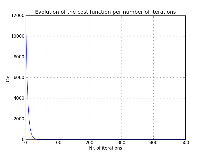
By applying feature scaling we can make gradient descent run much faster and converge in lot fewer iterations. When should the gradient descent algorithm be stopped? Manually: a plot should be done by having in the x-axis the number of iterations of the gradient descent algorithm and in the y-axis the cost:

The cost must always decrease after each iteration.

Automatically: it is possible to have an automatic convergence test - declare convergence if the cost J(θ) decreases by less than a small value ε (e.g.: 10-3) in one iteration - as it may be difficult to choose the value of ε, many times is better to plot the cost function has explained above.


Learning rate - α 


The cost function J(θ) should decrease after each iteration of gradient descent, but if it doesn’t, two things may be happening:

• there is a bug in the code - correct it
• the learning rate α is too high - decrease α

For a α which is small enough, gradient descent should always decrease, but if α is too small, gradient descent can be slow to converge.
To choose α we can try consecutively different values of α until we are satisfied with the result of the cost function: 0.001, 0.003 (=0.001 * 3), 0.01, 0.03, 01, 0.3.